Context/broader-outlook: vprog proposal.
The following presents a minimal formal model for the computational cost of synchronous composability for verifiable programs (vProgs) operating on a shared sequencer. The model defines a “computational scope”—the historical dependency subgraph a vProg must execute to validate a new transaction. The model shows that frequent zero-knowledge proof (ZKP) submissions act as a history compression mechanism, reducing this scope and thereby the cost of cross-vProg interaction.
1. The Model
Consider a system of vProgs interacting through a global, ordered sequence of operations.
-
vProg & Accounts: A verifiable program, p, is a state transition function combined with a set of accounts it exclusively owns, S_p. Only p has write-access to any account a \in S_p.
-
Operation sequence (T): The system’s evolution is defined by a global sequence of operations, T = \langle op_1, op_2, \dots \rangle, provided by a shared sequencer. An operation is either a Transaction (x) or a ZK-Proof Submission (z).
-
Transaction (x): An operation describing an intended state transition. It is defined by a tuple containing:
- r(x): The declared read-set of account IDs.
- w(x): The write-set of account IDs, with the constraint that w(x) \subseteq r(x).
- \pi(x): The witness set. A (potentially empty) set of witnesses, where each proves the state of an account a at a specific time t'. These are provided to resolve the transaction’s dependency scope and are independent of the direct read-set r(x).
-
ZK-Proof submission & state commitments:
- A proof object, z_p^i, submitted by
vProgp, attests to the validity of its state transitions up to a time t. It contains a state commitment, C_p^t. - Structure: This commitment C_p^t is a Merkle root over the sequence of per-step state roots created by p since its last proof z_p^{i-1} (e.g., from time j to t=j+k).
- Implication: This hierarchical structure is crucial because it allows for the creation of concise witnesses for the state of any account owned by p at any intermediate time between proof submissions.
- A proof object, z_p^i, submitted by
-
Execution rule: Any
vProgp that owns an account in w(x) must execute transaction x. -
Remark on composability: This execution rule enables two primary forms of composable transactions:
- Single-writer composability: The write-set w(x) is owned by a single
vProg, but the read-set r(x) includes accounts from othervProgs. - Multi-writer composability: The write-set w(x) contains accounts owned by two or more
vProgs. This implies a more complex interaction, such as a cross-vProg function call, and requires all owningvProgsto execute the transaction per the rule above.
- Single-writer composability: The write-set w(x) is owned by a single
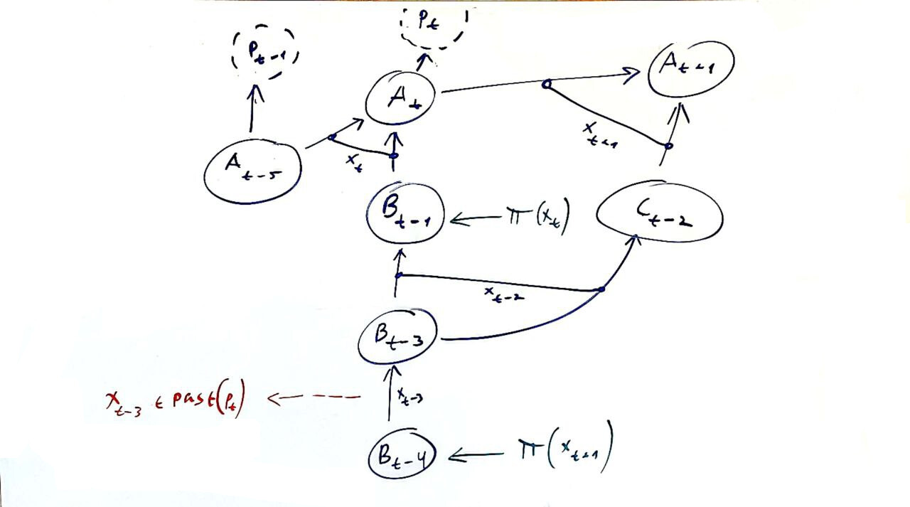
2. The Computation DAG
The flow of state dependencies is modeled using a Computation DAG G = (V, E), whose structure is determined dynamically by the global sequence of transaction declarations.
-
Vertices (V): A vertex v = (a, t) represents the state of account a at time t. The state data for a vertex is not computed globally; instead, it is computed and stored locally by a
vProgonly when required by a scope execution. -
Edges (E): The set E contains the system’s transactions. Each transaction x_t acts as a hyperedge, connecting a set of input vertices (its reads) to a set of output vertices (its writes).
-
Graph construction: When a transaction x_t appears in the sequence:
- New vertices are created for each account in its write-set, \{v_{a, t} \mid a \in w(x_t)\}.
- The transaction x_t itself is added to E, forming a dependency from the set of vertices it reads from to the set of new vertices it creates.
-
State compression: When a proof z_p^i appears in the sequence, it logically compresses the dependency history for all accounts in S_p. This creates a new, trustless anchor point in the DAG that other
vProgscan reference. The historical vertices are now considered eligible for physical deletion by nodes after a safe time delay. -
Remark on the write-set constraint: The rule w(x) \subseteq r(x), defined earlier, is enforced to ensure the DAG’s structure is independent of execution outcomes. If a transaction contains a conditional write to an account a_w \in w(x) that fails, the new vertex v_{a_w, t} must still be populated with a valid state. By requiring a_w to also be in the read-set r(x), we guarantee that the prior state of a_w is available to be carried forward.
3. Computational Scope
The scope is the set of historical transactions a vProg must re-execute to validate a new transaction, x_t.
-
Read vertices (R(x_t)): The dynamic set of graph vertices that the transaction’s declared read-set, r(x), resolves to at time t. For each account a \in r(x), this corresponds to the vertex v_{a,k} with the largest timestamp k < t.
-
Anchor set (A(p, x_t)): The set of vertices that serve as terminal points for the dependency traversal. For a
vProgp executing x_t, this set includes:- All vertices whose state is proven by a witness in \pi(x_t).
- All vertices for which p has already computed and stored the state data from a previous scope execution.
-
Scope definition: The scope is the set of historical transactions whose outputs are routable to the transaction’s inputs without passing through any known anchor. More formally:
Let \text{routable}(S, A) be the set of all vertices v from which there exists a path to a vertex in the set S that does not pass through any vertex in the set A.The set of vertices in the scope is then V_{scope} = \text{routable}(R(x_t), A(p, x_t)).
The Scope is the set of all transactions that created the vertices in V_{scope}.
Note: this set can be computed procedurally by a backwards graph traversal, e.g., BFS, starting from the vertices in R(x_t) where the traversal along any path is halted upon reaching a vertex in the anchor set A(p, x_t).
-
Remark on witnesses and anchor time: Unaligned proof submissions can create “alternating” dependencies. The hierarchical state commitment structure solves this by allowing a transaction issuer to choose a single, globally consistent witness anchor time, t_{anchor}, for all provided witnesses. This transforms the starting point for the scope computation from a jagged edge into a clean, straight line, limiting the scope to the DAG segment between t_{anchor} and t.
Core Contributions
This model provides a formal ground for several key properties of the proposed architecture, centered on sovereignty, scalability, and the emergence of a shared economy.
First, the model provides a formalization of vProg sovereignty. Despite the shared environment, vProgs retain full autonomy. Liveness sovereignty is guaranteed because a vProg’s ability to execute and prove its own state is never contingent on the cooperation of its peers. Furthermore, resource sovereignty is provided by the Scope function, which allows a vProg to price the computational load of any transaction and protect itself from denial-of-service attacks.
Second, the model provides a rigorous framework for analyzing computational efficiency and scalability, which is detailed in the following section. The key insight is that system-wide performance exhibits a sharp phase transition that can be managed by tuning the proof frequency to prevent the formation of a giant dependency component.
Finally, the Scope cost function serves as a primitive for a shared economy. It creates a positive-sum game of “dependency elimination,” where self-interested vProgs are incentivized to compress their history, making them cheaper dependencies for the entire ecosystem. It also provides a foundation for sophisticated economic mechanisms like scope-cost sharing or Continuous Account Dependency (CAD).
Scalability and Phase Transitions
System-wide performance is a direct function of the proof epoch length, F, which we define as the number of transactions between consecutive proof submissions. Assuming a globally coordinated proof frequency for simplicity, the total computational overhead does not degrade linearly but exhibits a sharp phase transition. This means efficiency is maintained by keeping the proof epoch length sufficiently short. The dependency entanglement within an epoch can be analyzed by reducing the timed computation DAG to a timeless, undirected graph G'_F, where vertices are accounts and an edge connects any two accounts that interact within a transaction. In this reduced graph, the size of the largest connected component serves as a proxy for the maximum aggregate scope a single vProg might need to compute.
The formation of this graph can be modeled using the well-known Erdős–Rényi random graph model. Let N be the total number of accounts and q be the probability of a cross-vProg transaction. A classic result for random graphs is the existence of a sharp phase transition: a “giant component” emerges if the edge probability p (proportional to Fq/N^2) exceeds the critical threshold of 1/N. To avoid this, the epoch length must be kept below this threshold, approximately F < N/q. For any F below this value, the largest dependency clusters are small, on the order of O(\log N). This result implies that the computational overhead becomes manageable. Instead of the worst-case scenario where a vProg re-executes the entire epoch’s history—a cost of O(nC), where n is the number of vProgs and C is the ideal cost—the work for an average vProg is the cost of executing its own transactions, plus a small, logarithmically-sized fraction of other transactions.
While real-world transaction patterns may be non-uniform, similar critical threshold phenomena are known to exist in more complex models like power-law graphs. The key insight remains: the model provides a formal basis for managing system-wide efficiency by tuning the proof epoch length F to stay within a region that prevents the formation of a giant dependency component. This efficiency mechanism is the foundation for the positive-sum game described earlier. Self-interested vProgs are incentivized to compress their history frequently, as doing so makes them cheaper and more attractive dependencies for the entire ecosystem. This economic pressure helps justify our initial simplifying assumption of a global proof epoch, as vProgs that fail to keep pace will effectively be excluded from composable interactions due to their high cost.