Context/prerequisite: Based rollup design
Notation glossary:
- H - a hash function, e.g. SHA256, or blake, (see discussion here re zk-friendly hashes)
- MT(x_1,x_2...,x_k) - the Merkle tree derived from x_1,...,x_k, with some implicit hash function H
- MR(x_1,x_2...,x_k) - the root of the above Merkle Tree
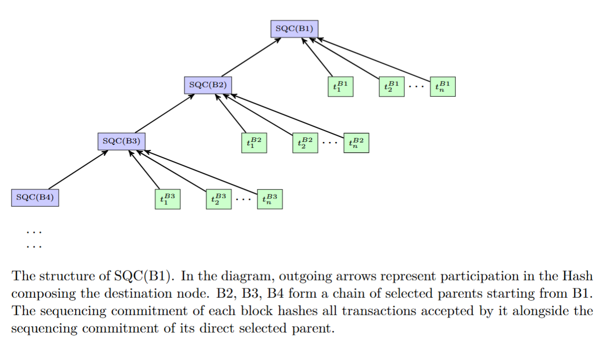
- SQC(B) - the “sequencing commitment” field of block B
- B.sp - the selected parent of the block B
Introduction
In Kaspa’s based rollup design we suggested introducing a new field, which serves as a sequencing commitment (previously referred to as the history root).
The new field is recursively defined as follows: let B be a block, and let t_1...t_n be all of B's accepted transactions (more accurately, the tx-hash or tx-id of those, to be determined at a later stage), in the order they were accepted in.
Ignoring initialization of the first block in the smart contracts hardfork, the new field SQC(B) is:
SQC(B)=H(SQC(B.sp),t_1, t_2...t_n),^1
as illustrated below:
To prove the progression of this field between a selected chain block Src and a selected chain block Dst matches the progression of the rollup, the prover requires all txs that were accepted between both of them as private inputs - inputs that the prover of a statement requires to produce a proof, but the verifier of that proof does not.
More formally, these are all txs that were accepted on a selected chain block in the future of Src and in the past of Dst, including Dst itself.
This scheme is perfectly functional, but it has the following inefficiency: a prover of a certain rollup, is really only interested in those txs that are directed to their rollup. All other txs, and any block that accepted no tx associated with this rollup, are “noise” from their point of view.
Yet in order to prove they are not associated with the rollup, provers are forced to take those as private inputs, increasing their runtime complexity.
In particular, if a rollup is only active once every 5 minutes, it would still have to go through the entire selected chain and all transactions accepted on it.
I explore below a method to represent a particular rollup history in a more concise manner.
Separate Subnet Histories
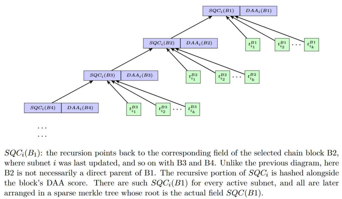
A rollup is represented by a field in the transaction called subnetId, and we refer to each rollup as a “subnet”. Our suggestion (courtesy of @michaelsutton) is that SQC have an inner structure representing the different subnets’ histories.
For a block B, and for each subnet i, let t_{i_1}...t_{i_k} be those transactions within B's accepted txs t_1, t_2...t_n that belong to subnet i.
We say a subnet i is active at block B, if there ever in history was an accepted transaction belonging to subnet i prior or at block B (this permanent definition of activeness will be relaxed below).
We can recursively define an abstract field: if block B accepted no txs of subnet i this field takes the same value as its selected parent, i.e. SQC_i(B)=SQC_i(B.sp).
Otherwise, SQC_i(B)=H(SQC_i(B.sp),t_{i_1},...t_{i_k}), or simply SQC_i(B)=H(t_{i_1},...t_{i_k}), if SQC_i(B.sp) was previously undefined. Lastly,
SQC(B)=MR(SQC_i(B)|\textit{i is active as of block } B),
meaning the Merkle root of the sequencing commitments of all active subnets.
The prover of subnet i now only requires the accepted txs between Src and Dst that belong to subnet i, as well as witnesses to prove the inclusion of SQC_i(Src), SQC_i(Dst) in SQC(Src) and SQC(Dst). These two witnesses are of logarithmic size in the number of subnets active in the network.
This prover now has O(A_i+\log R) private inputs, where A_i is the number of txs in subnet i at the span in between Src and Dst, and R is the number of active subnets. For some concreteness, with current parameters, \log R is at most 160.
The solution as is requires each L1 node to keep track of and compute SQC_i for all R subnets that are active, and subnets never become deactivated. Effectively this creates a “registry” of subnets. Thought must be devoted to prevent unlimited growth of this registry or spamming attacks.
I propose implementing pruning of the subnets: nodes will also store the last (selected chain) DAA score at which subnet i was updated, and subnets will only be considered active if the current DAA score is less than finality-depth greater than the last update on the subnet.
If subnets become indisputably inactive, their stored data can be thrown away completely during pruning. This ensures a bound on the number of active subnets at any given time.
Naive use of Merkle trees may result in recalculation of the entire tree at every block. To prevent this constant recalculation, I advocate using sparse Merkle trees.
For ease of syncing and general data tracking, SQC_i(B) should be updated to explicitly contain the last DAA score subnet i was updated at, e.g.,
SQC_i(B)=H(DAA(B),H(SQC_i(B.sp),t_{i_1},...t_{i_k})) whenever an update occurs.
A sketch of the structure of subnets history is provided below:
The pruning means that a subnet should make at least a single tx every finality-depth blocks if it wishes not to be pruned. Finality depth is planned to be about half a day after the 10bps hard fork. It appears to me like a reasonable requirement of a subnet to demonstrate its activity by issuing a tx every 12 hours.
Nevertheless, there is value in allowing a fallback mechanism in case that for whatever reason a subnet has been pruned prematurely. Hence I suggest we add another branch to SQC(B)'s sparse Merkle tree, called SQC_{TOT} (B)=H(SQC(B.sp),t_1,...,t_n) which stores the total history as originally proposed, without division to subnets and without pruning. That way pruned subnets could still supply proofs - at the cost of waiving all optimizations.^2 Another advantage of maintaining this divisionless branch, is that it maintains the original ordering of the accepted txs in their entirety, which may be required for some applications that choose to track all txs.
[1] Previously @michaelsutton suggested H(MR(SQC(B.sp),t_1, t_2...t_n)). The current reasoning to use a Merkle tree instead of a cumulative hash mostly reduces to overloading the new field with the responsibility previously kept by the Accepted Transactions Merkle Tree field, or possibly, the responsibilities of the Pchmr field proposed in KIP6 - if we later choose to implement a “logarithmic jumps” lookout into history instead of the linear one described here.
This kind of decisions are to be made at a later stage and I see fit to decouple them from the subject at hand.
[2] It is worth emphasizing that while a proof end point must refer to a relatively recent block for it to be valid, its starting point can be arbitrarily old.